What do you...mean...by expectation?

The post I probably should've written six months ago

I’ve written several posts about the expected value, or mean, of random variables. (For example: expected wait times, expected profit, inference for means.) Now that I’m teaching statistics from scratch, it occurs to me that it’s worthwhile to clarify what expectation means (pun—as they all are—very much intended).

The basics

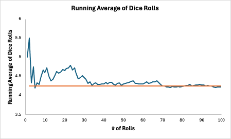
Ask anyone, and they can probably find the average of the four numbers: 5, 8, 1, and 4. Add them up and divide by the number of figures: (5 + 8 + 1 + 4)/4 = 4.5. If you instead asked for the mean of the four numbers, they would probably do the same thing (as they should). But what is the mean outcome for the roll of a die? This is a conceptual leap because you don’t have any pre-existing numbers to average. One way to explain it is to invoke the law of large numbers: the mean dice roll is the long-run average of N dice rolls as N gets bigger and bigger. I simulated 100 dice rolls in Excel, and the long-run average appears to be about 3.5:

The running average plotted as a function of the number of rolls. While the average is volatile initially, in the long run it settles near 3.5. This is the “law of large numbers.”

There are three problems (at least) with this definition:

1. We don’t want to have to run a simulation to compute every mean.

2. We don’t know if the long-run average even exists.

3. It’s unclear how many dice you have to roll before you can state the mean with confidence.

Evidently, we need a better method for finding the mean. To that end, note that the apparent mean of 3.5 for the roll of a die happens to be the average of the 6 outcomes:

\(3.5=\frac{1+2+3+4+5+6}{6}.\)

Before we jump to any conclusions, the formula can’t be that easy. What if, instead, the die that you’re rolling is loaded? For example, maybe 1, 2, and 3 each appear with probability 1/12, while 4, 5, and 6 each appear with probability 1/4.¹ This die has the same six possible outcomes, but it must have a larger mean. Why? The numbers 4, 5, and 6 are going to appear more frequently than they would for a normal die. I simulated this die as well and found the mean to hover around 4.3.

Rolling average for a die where 4, 5, and 6 are each three times as likely to appear as a 1, 2, or 3. The mean appears to be ~4.3.

Why does the mean of the unloaded die equal the average of the six possible rolls? The reason is that each outcome is equally likely (with probability 1/6). So, what looks like the average of the six outcomes is really the weighted average of the six outcomes, with the weights given by the probabilities. Explicitly:

\(\begin{aligned} \text{Mean}&=\left(\frac{1}{6}\right)\cdot 1+\left(\frac{1}{6}\right)\cdot 2+\left(\frac{1}{6}\right)\cdot 3\\[3pt] &+\left(\frac{1}{6}\right)\cdot 4+\left(\frac{1}{6}\right)\cdot 5+\left(\frac{1}{6}\right)\cdot 6\\[3pt] &=\frac{1+2+3+4+5+6}{6}=3.5 \end{aligned}\)

More generally, if you have a discrete random variable X, the expected value E[X] is defined as

\(E[X]=\displaystyle\sum_{\text{all }x}x\cdot P(x).\)

As a second example, let’s analyze the loaded die described above:

\(\begin{aligned} E[X]&=\left(\frac{1}{12}\right)\cdot 1+\left(\frac{1}{12}\right)\cdot 2+\left(\frac{1}{12}\right)\cdot 3\\[3pt] &+\left(\frac{1}{4}\right)\cdot 4+\left(\frac{1}{4}\right)\cdot 5+\left(\frac{1}{4}\right)\cdot 6\\[3pt] &=4.25 \end{aligned}\)

This also matches the simulation prediction.

If you’ve ever wondered why “the house always wins,” this is it. Each game in a casino is set up so that the expected winnings for the player are negative. Consider roulette. An American roulette wheel has 38 sectors: the numbers one through 36, plus 0 and 00. The 0 and 00 are green, and the remaining 36 numbers are evenly split between red and black. Correctly picking red or black pays 1:1. This means that if you bet $1 and win, your profit is also $1. What are the expected winnings for wagering $1 on red in roulette? There are two outcomes: either you win $1, or you lose $1. The expected value is

\(\begin{aligned} E[\text{winnings}] &=\$1\cdot P(\text{red})-\$1\cdot P(\text{not red})\\[3pt] &= \frac{18}{38}-\frac{20}{38}\approx-\$0.05. \end{aligned}\)

(Note that the two extra green spaces are what make this a bad deal for you. The expected payout for wagering $1 on black is the same.) How do we interpret this? If you wager $1 on red, you won’t lose a nickel. You’ll win $1 or lose $1. But, if you bet $1 on red 100 times, you should expect to lose about five more times than you win, which means you expect to be down ~$5.

If you have more-or-less unlimited money (like a casino), you can afford to offer people the chance to play this game. Even if someone goes on a heater—let’s say red comes up 10 times in a row—they know that they will make an average of $.05 on every $1 bet on red in the long run.² In fact, this model is so reliable for casinos that they’ll offer you free booze to keep playing. There are even a few bets in the casino with an expected value of $0 for the player (called “true” bets). The best example is craps, where the payout is 2:1 on a wager that repeated rolls of two dice will yield a 4 before a 7. You are twice as likely to get a 7 (6 combinations) as a 4 (3 combinations), so the 2:1 odds yields an expected payout of $0. The catch? In order to make this bet, you first have to place another bet where the house has the edge.

Continuous random variables

The previous section considered discrete random variables, meaning that you can list all the possible outcomes. (Note that this is different than finite, e.g. the Poisson distribution). How would you compute the mean of a distribution that is continuous, meaning that it takes values in an interval?

For continuous variables, we typically have a probability density function f(x). The nature of being continuous means that the probability of observing a specific value is 0. What’s the probability that a man is 70 inches? It’s 0%. One “70-inch-tall man” is really 70.1269385… inches. Another one is 69.9468648… inches. Thus neither is exactly 70 inches. Instead, we talk about the probability of lying in a range of variables. For example, the probability that a randomly chosen man is between 69 and 71 inches is not 0. To compute the probability, you integrate the probability density function over those values:

\(P(a<x<b)=\displaystyle\int_a^bf(x)\,dx.\)

Given that this is how we compute the probability, the expected value of a continuous random variable is what you would expect. Suppose X is a continuous random variable with density f(x) taking values in an interval [a, b]. Then the expected value E[X] is calculated

\(E[X]=\displaystyle\int_a^bx\cdot f(x)\,dx.\)

As an example, let’s consider the standard normal distribution. The word “standard” refers to the fact that the mean and standard deviation are 0 and 1, respectively. Thus, we know that the answer for expected value should be 0. To calculate it directly, we need the probability density function for the standard normal:

\(f(x)=\displaystyle\frac{1}{\sqrt{2\pi}}e^{\frac{-x^2}{2}}.\)

The normal distribution takes on all real values, so the mean is given by

\(E[x]=\displaystyle\frac{1}{\sqrt{2\pi}}\int_{-\infty}^{\infty}x\cdot e^{\frac{-x^2}{2}}\,dx.\)

If you’re so inclined, you can integrate that expression by finding an antiderivative.³ I prefer this argument: the integrand is an odd function (even exponential times odd polynomial), so the integral over any interval of the form [-c, c] is 0. (The two halves
[-c, 0] and [0, c] have the same magnitude but opposite signs.). This confirms that the expected value of the standard normal distribution is 0.

Some pathological examples

I’ll close as any good article should—with examples to give you nightmares. I mentioned earlier that one problem of relying on simulations to calculate means is that you don’t know if the mean exists or not. It turns out that even with a nice formula, the mean doesn’t always exist. I gave the example of the Cauchy distribution—a continuous random variable—in a prior article. Here’s another example that is discrete. Let’s say a random variable X takes on the values 1, 2, 3, … with probability

\(P(X=n)=\frac{c}{n^{2}}.\)

(You have to pick the value c so that the total probability sums to 1. The value is known, but it’s not important here.) The expected value of this distribution is

\(\begin{aligned} E[X]&=\sum_{n=1}^{\infty}n\cdot P(n)\\[3pt] &=c\sum_{n=1}^{\infty}\frac{n}{n^2}\\[3pt] &= c\sum_{n=1}^{\infty}\frac{1}{n}=\infty. \end{aligned}\)

The bottom sum is the “harmonic series,” which is known to diverge. This shows that both discrete and continuous distributions can have infinite means. This means that the long-term running average (cf., the dice pictures above) would not converge for a variable with this distribution.

I’ll finish with an unsettling gambling problem. Consider the following game. The house is going to keep flipping a coin until heads appears. If the first flip is heads, you win $2. Every time the casino flips tails, the pot doubles. For example, if the first flip is tails, then the pot doubles to $4. If the second flip is heads, you win $4. If it’s tails, the pot doubles again to $8. The question is: how much would you be willing to pay to play this game? Clearly, you would pay at least $2 because that’s the minimum prize. If we apply the logic of the roulette example above, you should be willing to pay up to your expected winnings from playing the game. If the game is k flips long, then the payout is 2^k. (That means the first (k - 1) flips were tails, so the original $2 prize doubled (k - 1) times.) The probability of a game lasting k flips is 1/(2^k), since a k-flip game specifies every single roll. Using the expected value formula, we see that the expected payout is:

\(\begin{aligned} E[X] &= \frac{1}{2} \cdot 2 + \frac{1}{4} \cdot 4 + \frac{1}{8} \cdot 8 +\cdots \\[3pt] &= 1 + 1 + 1 + \cdots \\[3pt] &= \infty. \end{aligned}\)

Since the expected payout is infinite, you should be willing to pay any amount to play this game! Would you pay $100,000,000? Breaking even at that price would require that the first 26 rolls are tails, and the 27th is heads. The chances of this happening are about 7 in one billion. This is where I remind you that I don’t give financial advice.

1. This is a valid probability distribution because 1/12 + 1/12 + 1/12 + 1/4 + 1/4 + 1/4 = 1.

2. It’s implied that the expected winnings to the casino are exactly opposite the expected winnings to the player. This wouldn’t be true in a game like poker, where there are players competing and the house takes a cut of each pot.

3. Interestingly, there is no antiderivative for the PDF itself. However, you can compute definite integrals for normal distributions—aka “Gaussians”—with a number of slick tricks.