When can't we use the central limit theorem?

A close look at one of the rare distributions to break the famous CLT.

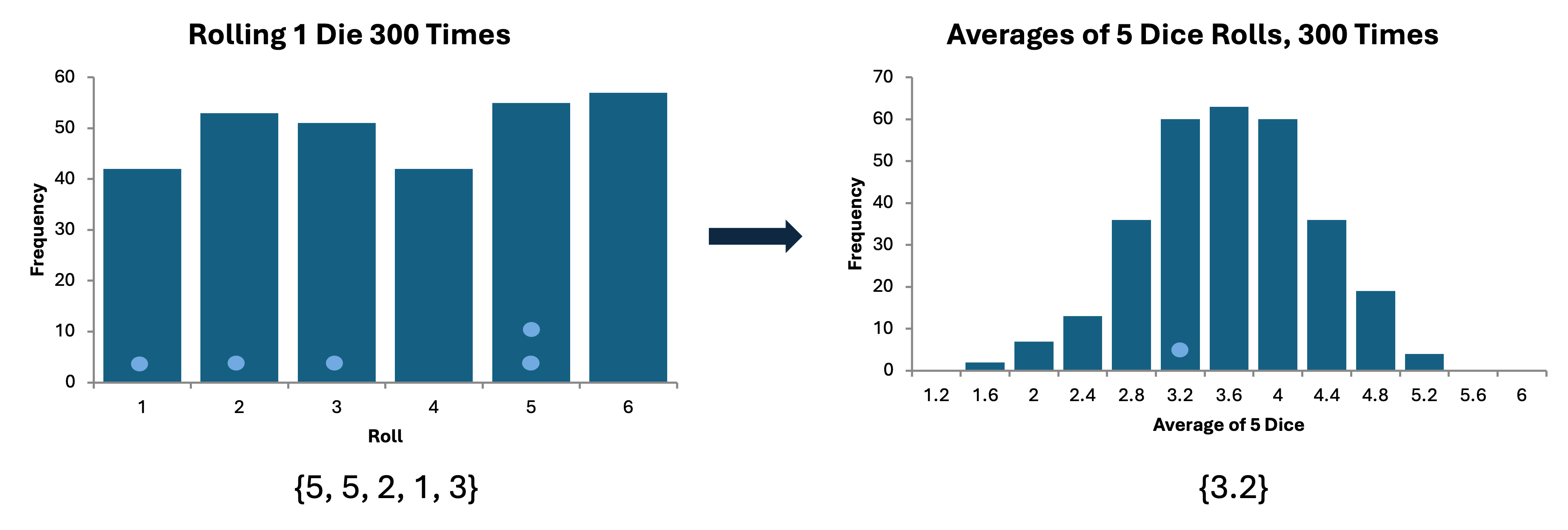
The central limit theorem (CLT) is the duct tape of statistics. In a nutshell, it says that if we repeatedly draw random samples from a population and take the mean of some feature of that population (e.g., height in inches, ounces in a can of soda, etc.), then these means will form a nice bell-shaped curve, provided the samples are large enough. The surprising part is that this is true regardless of how the underlying population is distributed. For example, suppose you roll a regular six-sided die and record the value. This has a uniform distribution: each number 1 through 6 has an equal likelihood of being chosen. Instead, what if we roll five dice and take the average of these rolls? Since each number is equally likely to appear for each roll, we expect the average to be (1 + 2 + 3 + 4 + 5 + 6) / 6 = 3.5. What the CLT says is that if we perform that experiment repeatedly—roll 5 dice, take the average, record the result, repeat—then the distribution of averages will be approximately normally distributed with mean 3.5. Since you should never just trust some guy on the internet, I simulated this experiment in Excel and made a histogram of the results.

Why is this helpful? Well, in a realistic scenario, the only way you can access a population is by sampling it. The CLT allows us to extrapolate from a sample to draw conclusions about the population. (This is called statistical inference.)

When does the CLT apply?

If you’ve ever taken statistics before, you know that people apply the CLT pretty liberally. “Sample size at least 30? Yes? Then you’re good to go! No? Just do it anyway!” The question I want to investigate in this post is whether there are populations whose structure make it impossible to apply CLT, no matter how large your samples are. To answer this, it’s helpful to look at a formal statement of CLT:

Central Limit Theorem: Let X be a random variable with finite mean μ and standard deviation σ. For sufficiently large sample size N, the distribution of sample means

\(\bar{X}=\frac{\sum_{i=1}^{N}X_i}{N}\)

will be approximately normally distributed with mean μ and standard deviation σ/√N.

How can we break the CLT?

To break the CLT, you might try to come up with a really pathological population. The normal distribution is symmetric, so maybe something extremely skewed? For example, you have a 1-in-292 million chance of winning the Powerball. It doesn’t get more skewed than that. Sure enough, if you play the lottery 2 billion times, you’d expect to win about 6.8 times, and the number of wins would be approximately normally distributed. Alas, skewness doesn’t do the trick. (The phrase “sufficiently large” gives a lot of leeway.)

To break the CLT, I’m going to focus on one sneaky word in the statement of the theorem: finite. Specifically, the premise of the CLT is that the underlying population has a finite mean and standard deviation. It turns out there are distributions for which this is not the case. The simplest example is probably the Cauchy distribution, which has the following probability density function (PDF):

\(p(x)=\displaystyle\frac{1}{\pi(x^2+1)}.\)

If you’ve taken statistics, you’ve encountered this distribution before; its alter ego is the Student’s t distribution with 1 degree of freedom. Here is a plot of the density compared with the standard normal distribution. (I used Knicks colors in honor of them recently clinching the 2 seed in the NBA playoffs.)

As you can see, the shape is similar, but the Cauchy distribution has “fatter tails.” This means that extremely large positive or negative values are much more likely. If you do the math (cf., the appendix below), you’ll see that the higher prevalence of extreme values makes the mean of the Cauchy distribution ∞.

If the mean of the Cauchy distribution is ∞, then what will happen when we create the distribution of sample means? The CLT would say that the blue curve should morph into the orange curve if your samples were large enough (scaled appropriately). As a test, I just generated 5 sample means with N = 100 in Excel.¹ The numbers I got were: -4.58, 1.05, -1.20, -30.25, -.63. Interesting — look at the 4th value. If you generated 100 values from the standard normal distribution and took the average, what are the chances of getting a number as small as -30? Applying the CLT, samples of size 100 from the standard normal distribution are also normally distributed, with mean 0 and standard deviation 1/√100 = .1. So a sample mean of -30 corresponds to a z-score of -300. To give you an idea of how unlikely that is, a z-score of -7 or smaller has about a one-in-a-trillion chance of occurring. The likelihood of -30 appearing is therefore unfathomably small. (ChatGPT claims 1-in-10^700, although I think it’s making that up.) This should be a clue that something weird is going on.

The idea behind the CLT is that your sampling distribution becomes more normal as your sample size increases. To test this for the Cauchy distribution, I simulated the sampling distribution in R for 5 different sample sizes: {1, 10, 50, 100, 500}. For a symmetric distribution—such as Cauchy—a sample size of 500 should be more than enough to get a “normal” shape. (Check out the dice-rolling example, which has N = 5.) For each sample size, I generated 50,000 sample means. I then used R’s density function to plot the probability density functions. I also plotted the standard normal distribution for reference. If the CLT worked, then you should see the density curves getting closer and closer to the standard normal as the sample increased.

Probability density functions for Cauchy sampling distributions and the standard normal. Plots were generated using R’s density() function, which uses kernel methods. Note that all of the Cauchy distributions are right on top of each other.

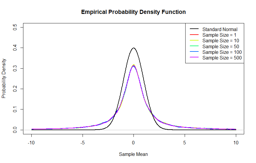
As you can see, the Cauchy sampling distributions did not approach the standard normal as the sample size increased. In fact, the sampling distributions were the same regardless of sample size. I find this remarkable. Think about generating a single Cauchy value. There’s a 50% chance that it’s positive, and 50% chance that it’s negative. You would think that if you average 500 of those numbers, the result would have to be closer to 0 than any single number itself. Maybe there are some extreme values on either side, but they should be canceled out by big numbers on the other side. Nope! Averages of Cauchy variables look exactly the same as single draws from the Cauchy distribution. If you’ve ever tried to create density curves out of histograms before, you might suspect that I cheated a little in the way I smoothed out these curves. (Actually, you would be right.) In case you need more convincing, you’ll see that we draw the same conclusion from looking at the cumulative density functions, for which there are no shenanigans.

Empirical cumulative density functions for samples of Cauchy variables, created using R’s ecdf() function. As before, the Cauchy sampling distributions are all right on top of each other.

There you have it. While the central limit theorem has definitely earned its reputation as the duct tape of statistics—capable of covering up almost any population flaw—it does have one Achilles heel. Next time you go to use it, make sure to ask yourself if your mean (or variance) could be infinite.

Appendix: Mean of the Cauchy distribution

In an attempt to quarantine the calculus in this post, I saved the calculation of the mean of the Cauchy distribution for the end. First, we should really verify that the Cauchy distribution is a valid probability distribution. To do so, we integrate the density function and make sure we get 1:

\(\begin{align}\displaystyle\int_{-\infty}^{\infty}\frac{1}{\pi(x^2+1)}dx & =\left.\frac{1}{\pi}\arctan x\right|_{x=-\infty}^{x=\infty} \\ & =\frac{1}{\pi}(\pi-0)=1.\end{align}\)

To calculate the mean, we integrate x times the probability density:

\(\begin{align}\displaystyle\int_{-\infty}^{\infty}\frac{x}{\pi(x^2+1)}dx & =\left.\frac{1}{2\pi}\ln(x^2+1)\right|_{x=-\infty}^{x=\infty} \\ & =\infty.\end{align}\)

Notice that on any finite interval [-a, a], the mean integral would be 0. This reflects the fact that the distribution is symmetric. However, the integral on the unbounded interval is infinite.

1. You can generate a single value from the Cauchy distribution in Excel with T.INV(RAND(),1). (The 1 refers to Student’s t with one degree of freedom.) I did this 100 times, and then took the average of those 100 numbers. I then repeated that experiment five times to get five sample means.