
Seeing the random forest for the decision trees
A look at two of the most useful and intuitive classification models.

I’m a little surprised that it took me 25 posts to get this one. This checks all the boxes: good math, widespread use in the business world, AND I teach it every quarter. As my MAC classes are about to dive into this subject again, I figure now is the time to finally write the post. The topic is decision trees and random forests. In the broadest sense, these are algorithms that help make decisions. I’m going to focus on the application of these models to classification, which is the task of assigning objects to different categories. I talked about classification in depth here, about metrics for assessing classifiers here, and about tuning parameters in classification models here.
Props to Kaggle
My earlier classification posts used a fictitious dataset from a company producing doodads. (Talk about beating a dead horse.) I was able to stretch that example as far as I did because I was focused on the outputs: namely, the class probabilities and the class assignment. For decision trees, there is more of a focus on the features of the objects in the dataset. For that reason, I decided to find a real dataset for this post. I checked out this site called Kaggle, which is an online machine learning community with resources including datasets. Don’t judge them by the name—this is a great site. Anyone can make a free account and access thousands of datasets with various criteria. For example, I filtered on datasets that are 1) suitable for classification, 2) scored a 10/10 on the ease of use scale (whatever that means), and 3) are related to business. I ended up picking a dataset related to customer churn at a bank. 10,000 customers are described in 11 dimensions:
Demographic data: country, gender, age
Financial data: credit score, estimated salary
Banking activity: total balances, tenure with the bank, number of products used, whether the customer has a credit card, and whether they are active
Churn: Has the customer left the bank (coded as 0 or 1)?
If you were this bank, you would want to be able to predict which customers will leave. Losing customers means losing revenue. If you could predict who will leave, then you could use targeted outreach to get those people to stay. On the flip side, if you knew who is likely not going to leave, you could probably cross-sell and up-sell more effectively. I’m going to show you how to use decision trees and random forests to predict who will leave. If you want to play along at home, I attached the dataset to the bottom of this post.
Decision trees
Of the 10,000 customers in the dataset, 2,037 have a churn value of 1, meaning that they left the company. If you picked a customer at random and needed to guess whether they left, what would you do? Absent any other information, the only thing you could do is play the numbers game—guess that they didn’t leave, given that only 20% of customers left. If you did this, there’s a 20% chance you’d be wrong. Nostradamus would’ve gone out of business with stats like that.
The goal of a decision tree is to segment your customer database so that you can improve your odds of guessing right based on which segment each customer falls in. A decision tree is basically a flow chart that assigns people to different buckets based on several tests. For example, here is a decision tree that I trained in Alteryx, the data analytics software that I teach at UNC.

Let’s see how this works. The first question is at the very top of the tree: is the customer in question younger than 43? If yes, they go to the left. If no, they go to the right. Let’s say a person is 38. The next question is whether they have less than 2.5 products at the bank (i.e., 0, 1 or 2). If that is true, then they go left again, which leads all the way down to the dark blue bucket in the bottom left. At the top of that bucket you see the number 0. That means that everyone in this bucket gets assigned a churn value of 0 (i.e., not leaving). This is our first customer segment: people who are younger than 43 who use two or fewer of the bank’s products. For any customer with this profile, we will predict that they do not leave the bank. The fraction at the bottom of the box gives the proportion of people in the bucket who did not churn. Explicitly, there are 4,872 people with two or fewer bank products who are younger than 43. 4,362 of these 4,872 (89.5%) did not churn. Since we predict that everyone with this profile will remain, we would be right 89.5% of the time. This is a solid improvement over our 80% success rate for guessing no for everyone.
What makes for a good bucket? Evidently, we want everyone within a bucket to have the same churn value. Remember that this the only information we have to go off of, so we must make a uniform choice for the entire bucket. The greater the proportion of people who share the majority churn value, the more accurate our prediction for that bucket will be. We use the notion of entropy to describe how homogeneous or heterogenous a bucket is with respect to the variable we are trying to predict.1 A bucket has low entropy if the churn values are mostly the same (good), and high entropy if there are lots of people who left and lots who stayed (bad). There are a few different algorithms for building decision trees, but the main idea for all of them is to see what happens to entropy when you try different combinations of variables to define your buckets.2 The change in entropy is called information gain. If a tree has high information gain, it means that the buckets in the tree are more homogeneous than your original dataset. Accordingly, predictions made using that tree will be much better than just predicting that no customers will churn.
Random forests
If you asked a 5-year-old how a random forest differs from a decision tree, they would probably guess correctly. A random forest is just a bunch of trees. The forests are random in a few ways. First, each tree is built on a random subset of the data. Additionally, forests use a random subset of features (i.e., variables) when deciding what test to use for each decision point. For example, in the decision tree shown above, all variables were considered before deciding that {products < 2.5?} was the optimal question to ask a person younger than 43. By contrast, for one tree in a random forest, the algorithm might only look at three variables (e.g., number of products, age, and country) when designing a test for a given branch in the flow chart. What’s the point of looking at only chunks of your data at a time? For starters, it speeds up the algorithm. A random forest might have 500 trees, each of which needs to be trained. Reducing the volume of data—in both the number of rows (customers) and columns (customer features)—reduces the computational burden.
The other benefit of using random subsets of the data for training different trees is that it encourages diversity. To see why this is important, I should talk about how random forests assign customers to segments. For decision trees, it’s pretty straightforward: you flow them through the tree and see where they end up. It’s like the game Plinko from the Price is Right. This doesn’t make sense for forests because there is no single tree. Instead, a random forest is a “council of trees.” (Doesn’t that sound like something from the Lord of the Rings?) To make a prediction with a forest, you flow a customer through each tree and see if they come out as churn or stay. Then you have to figure out how to roll up the outputs from each tree. There are a few ways you can do this. The naive way is to take the majority opinion: if a forest has 300 trees, and 151 of them say that a customer will churn, then predict churn. It turns out that this simple method is the most common in practice.
Should you use a tree or a forest?
Let’s get back to the issue of diversity. In the tree I’ve been using, the variable products_number—specifically, the test {products_number < 2.5}—dominates the tree. The left-most bucket contains 4,872 customers, which is 69.6% of the 7,000 used for training the tree. The only tie that binds people in this bucket is that they’re younger than 43 (most of the customers) and have fewer than three bank products (also most of the customers). As mentioned earlier, the job of a decision tree is to pick features and questions that lead to buckets that are as homogeneous as possible. The problem is that over-relying on certain features can lead to overfitting: an undesirable situation where a model performs well on the data used to train it but doesn’t generalize well to new data. It turns out that decision trees are pretty much guaranteed to overfit. By contrast, random forests avoid this issue by randomly selecting only certain features for each decision point in a tree. While many of the decision trees in a random forest will feature products_number, others will leave that feature out, which means that they’ll be forced to learn other important factors for predicting churn. The hope is that this will help the random forest perform better when it sees new data.
To test this idea, I trained a decision tree and a random forest on 70% of the customers, reserving 30% for testing (i.e., assessing performance on new data). The decision tree outperformed the random forest on the training data for each of accuracy, precision, and recall. (Check out this article for a refresher on those terms.) This is not surprising. As I mentioned earlier, the decision’s tree’s raison d'être is to make great predictions on those specific customers. The random forest is a collection of decision trees, each of which is worse at making predictions than the single decision tree. Therefore, holding a vote among those trees to predict whether a customer will churn is probably not going to produce a better outcome than the primo tree. (I’m sure there’s some parable about democracy in there.) On the other hand, the reverse is true when you look at test set performance. To best way to visualize the superior performance of the random forest is by drawing a ROC curve. As a reminder, a ROC curve shows the trade-off between true positive rate (TPR) and false positive rate (FPR) for different churn thresholds. (Both trees and forests output probabilities that a customer will churn. You can change the threshold for classifying a customer as churn, which is how you trace out these curves.) Once you get beyond a TPR of ~50%, we see that the decision tree will have to tolerate many more false positives to achieve an equivalent true positive rate to the random forest.

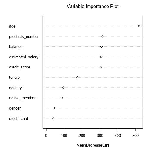
It’s pretty universal that a random forest will outperform a decision tree on new data. In real life, performance on the test set is all that matters. For that reason, random forests are more common. (Remember, machine learning is a results-oriented business.) However, decision trees can still be good for getting a handle on which variables may be important. For example, our tree first split on age, and next on the number of products. Alteryx (leveraging R) has something called the variable importance plot, which shows how much discriminatory power each feature brings to the party for a random forest. As we can see, these variables were most important in the forest too, which is comforting.
I hope you enjoyed reading this introduction to decision trees and random forests. Please subscribe for more content like this.
“Entropy” is my pick for the second-most abused term in STEM. It’s used in so many contexts, in slightly different ways, that it’s difficult to keep track of them all. If you’re wondering, #1 is “protein.” It seems like EVERYTHING is a protein. You’re telling me nothing by calling something a protein.
Instead of entropy, some algorithms—mostly older ones—use something called Gini impurity. Both measure homogeneity, and the difference isn’t important here.