How good is your classification model?

Some metrics and rules of thumb for assessing performance of a classification model.

A few weeks back, I wrote that naive Bayes classifiers are surprisingly good at their job. This week, I want to say more about what it means for a classifier to be good at its job. In short, it depends on what you’re trying to predict and why. Let’s jump in.

Doodads revisited

Are you sick of doodads yet? I hope not, because I’m planning to milk this example until they kick me off Substack. As a reminder, the company that manufactures doodads developed a naive Bayes (NB) classifier that predicts whether a doodad is good or defective early in the production process. This is an example of a binary classification problem, meaning that there are two outcomes: good or defective. If you make such a prediction, there are exactly four things that can happen:

• You predict good, and the doodad is good.

• You predict good, but the doodad is defective.

• You predict defective, but the doodad is good.

• You predict defective, and the doodad is defective.

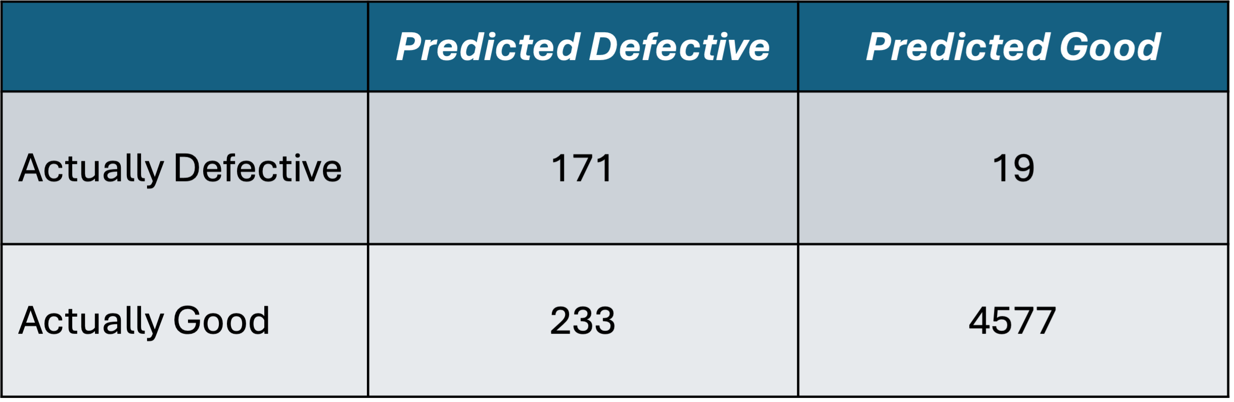
It is common to organize these outcomes in a 2x2 table called a confusion matrix.¹ For example, the confusion matrix for an NB classifier making predictions on 5,000 doodads might look like this:

Confusion matrix for a hypothetical classifier of doodads as good or defective.

How do we know if this classifier is doing a good job or not? The intuitive thing to do is to check what percentage of doodads are classified correctly. This is called accuracy. To generalize things, let’s refer to a prediction of “good” as a positive prediction. That makes “defective” a negative prediction. (Choosing “good” as positive instead of “defective” is arbitrary.) We can now re-write our four possible outcomes with this terminology.

• True positive (TP) = You predict good, and the doodad is good.

• False positive (FP) = You predict good, but the doodad is defective.²

• False negative (FN) = You predict defective, but the doodad is good.

• True negative (TN) = You predict defective, and the doodad is defective.

The “true” predictions are the accurate ones, so we have

\(\begin{aligned} \text{Accuracy} &= \displaystyle\frac{TP+TN}{TP+TN+FP+FN} \\[1em] &= \displaystyle\frac{4,577+171}{5,000} = 94.96\%. \end{aligned}\)

The denominator includes all 5,000 predictions because we want to know what percentage of all predictions are correct. Accuracy is one example of a metric. A metric is a number that measures the performance of a statistical model. Metrics can be used to help train models and to compare two models against each other.

It’s important to remember that we don’t classify for classification’s sake. The company built this model to inform its decision making. Specifically, if the classifier predicts that a doodad is good, it will ship that doodad to a customer. If the classifier pegs a doodad as defective, it will abort production on that doodad and write off the materials. Making a bad prediction has consequences. Suppose you have the following information from the finance department. The lost profit margin from discarding a good doodad because you believe it to be defective is $10. On the other hand, each defective doodad that is shipped to a customer costs the company $100 in the form of an apology VISA gift card. Another way to say this is that the cost of a false positive—predicting that a doodad is good when it is really defective—is $100. Conversely, the cost of a false negative—predicting that a good doodad is defective—is $10.

In light of this new information, is accuracy the best metric for assessing our predictive model? Accuracy does not distinguish false positives from false negatives. We know that 252 of our predictions are false (5.04%). Whether that is 252 false positives, 252 false negatives, or some combination of the two, accuracy does not change. Instead, the cost asymmetry in this case may lead us to prioritize minimizing false positives. How does this translate into a metric? It turns out that there are two directions you can take this, which give slightly different metrics. One is to make sure that you are catching as many of the defective doodads as possible. Defective doodads are those in the “negative” class, which includes true negatives and false positives. The true negative rate (TNR) is the percentage of these that are true negatives:

\(\begin{aligned} \text{TNR} &= \displaystyle\frac{TN}{TN+FP} \\[1em] &= \displaystyle\frac{171}{171+19} = 90\%. \end{aligned}\)

This is the natural language of a quality control system: we can correctly identify 90% of defective doodads. The other direction you can go is to focus on your predictions, not the actual state. In other words, among the doodads that you identify as good, what percentage are actually good? This is called precision:

\(\begin{aligned} \text{Precision} &= \displaystyle\frac{TP}{TP+FP} \\[1em] &= \displaystyle\frac{4,577}{4,577+19} = 99.59\%. \end{aligned}\)

In either case, you are penalized for having more false positives, as FP appears in the denominator. Therefore, these would be good metrics to choose if your goal is to minimize false positives. How do you decide between the two? As we see here, precision is off the charts. Is this because our classifier is awesome? Not really. The reason that precision is so high is because most of our doodads are true positives. In fact, most doodads are positive (i.e., good) regardless of our prediction. Per the confusion matrix, the percentage of good doodads is (233 + 4,577) / 5,000 = 96.2%. This means that if we simply predicted that every doodad was good, our precision would be 96.2%. One of the important features of a performance metric is that it is discerning. For example, if everyone got 1600 on the SATs, they wouldn’t be useful to universities. (This is not a pro- or anti-SAT post.) Given that, my preference would be to use the true negative rate in this case. (However, I think that practitioners tend to default to precision.)

While the costs in the doodad example spurred us to avoid false positives, there are other cases where false negatives are more consequential. For example, you would want to minimize false negatives for any medical diagnostic where the condition is deadly if you fail to diagnose. For such problems, the correct metric to use is called recall, also known as the true positive rate or sensitivity. It answers the question: what percentage of good doodads did you predict to be good?

\(\begin{aligned} \text{Recall} &= \displaystyle\frac{TP}{TP+FN} \\[1em] &= \displaystyle\frac{4,577}{4,577+233} = 95.15\%. \end{aligned}\)

Accuracy, precision, and recall are probably the “Big 3” when it comes to classification metrics. However, I want to discuss one more common metric called F1-score. I mentioned above that the precision vs. true negative rate choice may be influenced by having heavily imbalanced data (i.e., actual positives far outweigh actual negatives or vice-versa). What if you have an imbalanced dataset, but you don’t want to prioritize one of FP or FN? F1-score addresses this by taking the harmonic mean of precision and recall:

\(\begin{aligned} F1\text{-score} &= \displaystyle\frac{2}{\frac{1}{\text{Precision}}+\frac{1}{\text{Recall}}} \\[1em] &= \displaystyle\frac{2\cdot\text{Precision}\cdot\text{Recall}}{\text{Precision}+\text{Recall}} \\[1em] &=\frac{2\cdot(.9959)\cdot(.9515)}{(.9959)+(.9515)}=97.32\%. \end{aligned}\)

The harmonic mean, as opposed to the straight average (aka arithmetic mean), is frequently used to take averages of rates or ratios, of which precision and recall are examples. F1 is less sensitive to imbalanced datasets because precision and recall are already themselves ratios, so it’s harder for one square of the confusion matrix to dominate. (Actually, the one exception is TP, so F1-score is most useful when the TP class is smaller; since you are free to choose the positive class, this is not a big problem.) It’s worth mentioning that F1-score has passionate detractors. Nonetheless, it’s a common metric to look at in classification.

Conclusion

In this post, we covered the four primary metrics for analyzing classification algorithms:

• Accuracy = Percentage of objects that you classify correctly

• Precision = Percentage of the objects you classify as positive that are actually positive

• Recall = Percentage of positive objects that you predicted as positive

• F1-Score = The (harmonic) average of precision and recall

Accuracy and F1-score are good if you don’t care more about false positives than false negatives (or vice-versa). Use the latter if, in addition, your dataset is heavily imbalanced between actual positives and actual negatives. If your priority is to minimize false positives, use precision. Finally, if your priority is to minimize false negatives, then use recall. I hope you enjoyed reading. Please subscribe and share with your network.

1. If you have a multi-class problem—that is, a classification problem with more than 2 classes—you can still make a confusion matrix. In general, if there are n classes, then the confusion matrix will be an n x n table. However, the n = 2 case is the only one where we can easily define true positive, false positive, true negative, and false negative.

2. In statistics, false positives are called Type I errors, and false negatives are called Type II errors. False positive (resp. negative) is more common for classification problems, whereas Type I error (resp. Type II error) is more common in hypothesis testing.