
Naive Bayes Classifiers
A lightweight, yet very effective, classification tool

Classification is the process of assigning objects to different categories based on their characteristics. For example, suppose you want to determine if an email is spam. You could encode each email using several features: word count, frequency of buzzwords like “free”, number of spelling errors, etc. Further, if you had examples of spam and non-spam emails, you could then train a model to recognize which features tend to indicate spam. This process is called supervised learning: you give your model the “answer key” for the practice emails, hoping that it will be able to use them to figure out how to classify new emails.
Naive Bayes (NB) classifiers are among the simplest supervised learning models used for classification tasks. Despite their simplicity, in many cases they can still hang with the “big boys” of classification, such as deep neural networks and random forests. I’ll talk a little bit about why this is at the end of the post. For now, let’s start with an example to understand how NB classifiers work. You will need to know the basics of conditional probability, which you can read about here.
Predicting defective doodads
Last week, a hypothetical manufacturing company was about to implement a new quality control system that would help it identify defective doodads. While the QC system works well, it can’t analyze a doodad until after the lengthy production process. Now the company wants to push the envelope and see if it can identify defective doodads earlier in the process, thus allowing them to abort the process early and save production costs. Suppose they sampled a few defective and non-defective doodads and recorded the following information about the doodads after step 1 of the production process:
Weight of the doodad in grams,
The shift that production began (morning or evening), and
Whether the machine was properly calibrated for step 1.
Here’s the data.

The Bayesian probability model
The principle underlying NB classifiers is pretty simple. Each doodad is either good or defective. For a given doodad, the goal is to determine which of those categories is more likely, and then classify it as such. Given the data that we have, you can describe each doodad with a vector of features x = (shift, machine status, weight). For example, one doodad might be (morning, mis-calibrated, 501). The two probabilities we need to calculate are therefore the following:
The expressions on the righthand sides are direct applications of Bayes’ rule. At first glance, we just made the problem three times harder. However, we can simplify things. Let’s start with the denominator, which is the same for both classes. Since our task is to determine which of P(good|x) and P(defective|x) is bigger, it makes no difference if we divide by P(x). We are therefore free to ignore it.
Next, what about P(good) and P(defective)? In Bayes speak, these are called the prior probabilities or priors. Why prior? Because they are the probabilities of being in each class prior to observing the evidence x about the doodad. (Similarly, the values P(good|x) and P(defective|x) are called the posterior probabilities because they represent the probability of being in each class after observing the evidence.) In practice, a few things might happen with the priors. Sometimes, you have good estimates of them. That is the case here, for example. In last week’s article, we said that P(good) = .96, and P(defective) = .04. These are accurate figures built upon years of observations of doodad production. More often, we either assume equal class probabilities or use the data to determine the priors. In this case, those two methods give the same answer. Our sample has 4 defective doodads and 4 good ones, so you could use P(good) = P(defective) = .5. Naturally, the sensitivity of NB classifiers to assumptions about the priors gets a lot of research attention. My impression is that it typically doesn’t make or break model performance, but I’m neither an expert nor a frequent practitioner.
Now we come to the heart of the matter: P(x|good) and P(x|defective). The challenge with these is that x is a three-dimensional vector—shift, machine status, and weight. (In real-world applications, these vectors could be massive.) If we want to estimate these probabilities (called joint probabilities), then we have to consider all possible combinations of these variables. For example, suppose you instead had 20 features, each of which were yes/no. (By today’s standards, this is still a very small model.) The joint distribution has 2^20 > 1,000,000 possible outcomes. To get a reliable estimate of the probabilities, maybe you have to collect 10 times that many samples. Then double that for each of the outcome classes. When was the last time you worked with a dataset with over 20,000,000 rows in it?
To get around this issue, we make the following assumption: conditioned on class, the features shift, machine status, and weight are independent.1 In math-ese:
(The analogous formula holds for P(x|defective).) Why is this an improvement? The reason is that we can look at each variable separately to estimate the probabilities. Let’s look at the example of machine status. Of the four “good” doodads, three had a machine status of proper, and one had a status of mis-calibrated. Of the four “defective” doodads, two had a machine status of proper, and two a machine status of mis-classified. This gives us the following probabilities:
P(proper|good) = 3/4
P(mis-calibrated|good) = 1/4
P(proper|defective) = 1/2
P(mis-calibrated|defective) = 1/2
Let’s think about scaling this. If you had 20 binary features, as above, then the number of probabilities that you need to estimate is 20 (features) * 2 (possibilities) * 2 (class categories) = 80. That’s a total steal compared to the 2M+ needed for the full joint probability distribution. This is why NB classifiers are used a lot in text analysis or natural language processing (NLP) applications. Typically, feature representations of text are very high-dimensional. (That’s a topic for another day.) The computational complexity of NB classifiers grows linearly in the number of features, which is pretty rare.
Keeping in mind that there’s no such thing as a free lunch, we should stop to scrutinize the independence assumption a little bit. To decompose the joint probability like we did requires that all three features are independent among good and defective doodads. Does this make sense? Take machine status and shift, for example. If one shift had more defective doodads than another, one reason might be personnel on the clock during each shift. But wouldn’t the person operating the machine also impact how likely the machine is to be properly calibrated? That would suggest dependence between machine status and shift, which violates our assumption. In practice, this happens a lot, especially for data with a large number of features. At the end of the post, I’ll talk a little about why people have success using NB classifiers despite this apparent limitation.
Gaussian naive Bayes
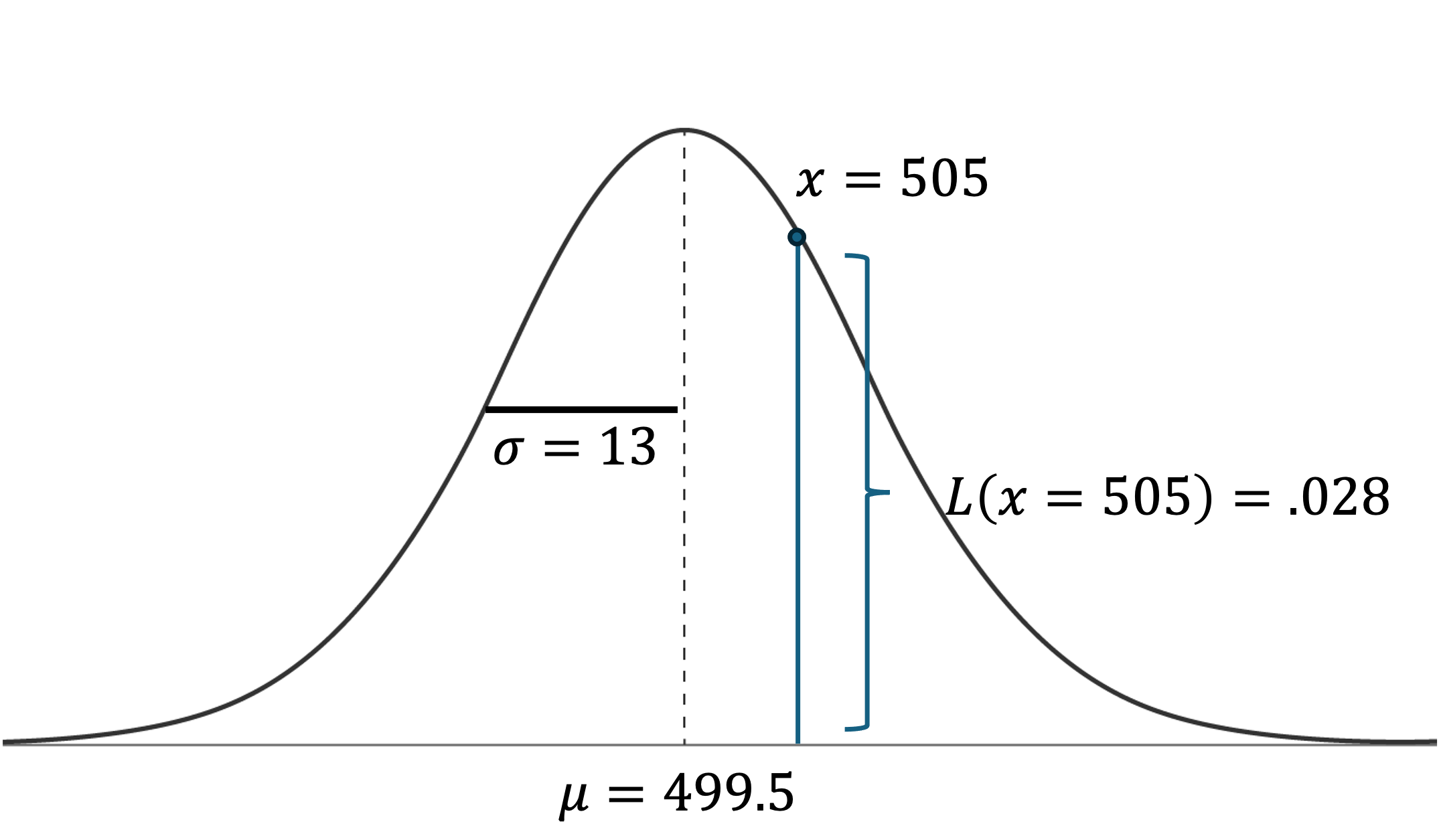
I calculated the conditional probabilities for machine status earlier. You can apply the same reasoning to get the probabilities for morning and evening shift as well. But what about weight? The weights of the defective doodads are 490, 500, 483, and 498. Does that mean we assign each of them probability 1/4? That would not be a good approach. Weight is really a continuous variable, so we should reflect that in the probability calculation. One way to do this is to “discretize” weight, which means to force weight to be categorical by creating different bins of weight (e.g., 490-493 grams). Then you could assign a probability based on frequency, as above. A better way to handle continuous data is to model it using a probability density function. The simplest example would be a Gaussian, or bell-shaped curve.2 We then end up with a two-step process. Step 1 is to find the Gaussians that best model weight for each class. Step 2 is to compute the likelihoods for each weight based on those Gaussians.
A Gaussian (aka normal distribution) is fully described by its mean and standard deviation, so we just have to compute those values for the weights of each of defective and good doodads. With the help of Excel, I found that defective doodad weight has a mean of 492.8 g and a standard deviation of 7.8 g, whereas good doodads have a mean weight of 499.5 g with standard deviation 13 g. To find the likelihoods, you just have to find the values of the probability density at that point. For example, to find L(weight = 505 | good), you can type NORM.DIST(505, 499.5, 13, 0) in Excel. The 0 tells Excel that you want the y-value on the density curve, not the cumulative area under the curve up to that point. (If you’re playing along at home, the answer is .028.)
You may have noticed that I did something sneaky: I switched from P( ) to L( ). The reason for this is that for continuous variables, the probability of being exactly 505 g is 0. To get nonzero probabilities, you need to take a range of weight and find the area under the curve between those weights. By using the notation L, I am switching from probabilities to likelihoods, which is common parlance for Bayesian things. The difference is subtle, but important. While it is true that the probability of having a good doodad with weight 505 is 0, we can talk about the relative likelihoods of having a good doodad with weight 505 vs. a defective doodad with weight 505. To convince yourself of this, put a really small interval of width ε around 505. The probability of a good doodad having weight in that interval is approximately ε*L(505, good)—base times height. Likewise, the probability of a defective doodad having weight in that interval is approximately ε*L(505, defective). In the ratio, the ε cancels out, and we see that the relative likelihood is determined by the density function at 505.
With that detail out of the way, we can compute the marginal probability distributions for our sample data.

Bringing it home: the decision step
So far, we’ve managed to build a Bayesian probability model for the posterior probabilities of good and defective doodads. To make this a classifier, we need to pair the probability model with a decision. The most natural decision is to assign the class that has the highest posterior probability: the maximum a posteriori (MAP) rule. Let’s see how this works on a new doodad x with weight 490 g, which was produced during the evening shift, and for which the machine was properly calibrated. Using the prior estimate of P(good) = .96 and the independence assumption to decompose P(good|x), we get:
In order, the terms on the right are P(evening shift|good), P(proper|good), L(weight = 490g | good), and P(good). I calculated the last term using NORM.DIST(490, 499.5, 13, 0). That symbol that looks like a fish means “is proportional to”; we lose the = because I left off the denominator, which we said earlier does not impact the decision. The analogous calculation for P(defective|x) is:
So how do we classify this doodad? We see that
Since it’s almost 8 times more likely that this doodad is good than defective, we classify it as good. I’ll point out that the prior assumption—the 4% defect rate—makes a difference here. If we did the typical thing of assuming equal prior probabilities, then the ratio would have been 8.8*(.04/.96) = .37, which is less than 1. In other words, without knowing that good doodads have a much higher prevalence than defective ones, the evidence in this case would have pointed to this doodad being defective.
Why do naive Bayes classifiers work so well?
I’ve already talked about how strong of an assumption conditional independence is among predictors. In most cases, we can point to at least one pair of predictors for which this assumption is clearly false. Take the Wikipedia article on naive Bayes classifiers, for instance, which gives an example of predicting gender using height, weight, and foot size. Clearly, weight and foot size both increase (on average) as height increases, so these are heavily co-dependent.
If the fundamental assumption underlying NB classifiers is bogus, why do they work so well? Many people have researched and written about this topic. To me, the most satisfying explanation comes from Domingos and Pazzani.3 The crux of their argument is that NB classifiers can be good in two ways. First, the posterior probabilities for each class can be accurate. Second, the NB classifier can come up with accurate predictions of each class. Of course, if your classifier is good at the former, it’ll be good at the latter, since the probabilities are used to make classifications. However, the reverse is not true. In principle, your posterior estimates could be pretty bad, but as long as the largest posterior probability is the correct class, you’ll get away with it. Here’s an example.

Domingos and Pazzani argue that using a so-called 0-1 loss function—that is, judging your model’s performance based on the number of misclassifications—explains why NB classifiers perform so well despite violations of the independence assumption. This argument is supported by empirical evidence showing that NB classifiers tend to produce poor probability estimates, even though their classifications are accurate. Another explanation for NB classifier success is that they perform well due to the way dependencies are distributed across classes (e.g., they may “cancel out”).4 Either way, if you ask me, classification is a results business. If you can get the right answer with one of the computationally cheapest models around, more power to you.
Recap
This post reviewed naive Bayes (NB) classifiers. Here are the key takeaways:
NB classifiers are extremely efficient and suitable for very high-dimensional datasets, such as text-related applications (spam filtering, document classification, etc.).
The “naive” assumption made with NB classifiers is that the features are mutually independent, conditioned on class. Although this assumption is false in almost every case, the resulting models still work well in practice.
Using the ratio of posterior probabilities (i.e., P(good|x) / P(defective|x)) allows us to blend discrete predictors (based on probabilities) with continuous ones (based on likelihoods).
Thank you for reading. Please subscribe and share with friends.
Note: Conditional independence is not the same as independence. Neither independence nor conditional independence implies the other. That is, you could find A, B, and C such that P(A and B) = P(A)*P(B)—i.e., A and B are independent—but P(A and B|C) does not equal P(A|C)*P(B|C) and vice-versa.
Kernel density estimates are a way of fitting non-Gaussian density curves. Wikipedia claims that doing this can greatly improve NB classifier performance.
The optimality of naive Bayes, Harry Zhang