


What is a confidence interval?

If you’ve ever taken statistics, you know that things start to get weird when you get to the unit on inferential statistics. As the name suggests, inferential statistics is about jumping to conclusions (i.e., making inferences) based on a random sample of some population. These inferences come in two flavors:
Confidence intervals: finding a range of values within which we’re pretty sure that a population parameter lies.
Hypothesis tests: deciding if there is enough evidence to reject an assumption about a population parameter.
The population parameter is usually a mean or proportion, but it could also be a variance or several other things. As an example, a mean might be the average height of people in some country. A proportion could be the percentage of people who are in favor of a particular ballot measure in a community.
In this post, I want to shed some light on what a confidence interval is. First, let’s assume we have the following basic ingredients:
Unknown population mean:

Sample mean:

Margin of error:

Confidence level:


With this set up, the lower bound of the confidence interval is 3 (= 5 – 2) and the upper bound is 7 (= 5 + 2). On the AP Statistics exam, you would be asked to interpret the confidence interval. If you studied hard, this is what you would write:
We are 95% confident that the true population mean is between 3 and 7.
That response would get full credit. But what does it actually mean? A reasonable guess would be that there’s a 95% chance that lies somewhere between 3 and 7. Unfortunately, this is not quite right. The population mean is a fixed, albeit unknown, number, so it’s either between 3 and 7 or not.
To better understand confidence intervals, I want to leverage an earlier post about estimating the mathematical constant π. In that article, I used Excel to randomly pick points in a square, and then I calculated the percentage that also lie in an inscribed circle. From the area formulae for squares and circles, we knew that the proportion of points lying in the circle should be π/4, which is about 78.5%. (That article has a picture of the scenario.)
Now I want to look at this experiment from a different perspective. If we randomly pick points in the square, say 500 of them, we can think of the proportion lying within the circle as a sample proportion, which estimates the true population proportion of p = π/4. I got a sample proportion of p-hat = .792 (396 out of 500) when I did this the first time. Let’s put a 95% confidence interval around this value by computing the margin of error. You can find the formula here.
}{n}}=(1.96)\cdot\sqrt{\frac{.792\cdot .208}{500}}=.0356.")
Subtracting and adding this number from .792 gives us a confidence interval of (.756, .828). Where does 95% come in? It’s encoded in the number z_crit = 1.96. As the confidence level increases, z_crit increases as well, which means that confidence intervals must be bigger to accommodate higher confidence. For a given level of confidence C, you can find z_crit in Excel with the function NORM.S.INV(1-.5*(1-C)). Now I can explain what a confidence interval means:
If you repeatedly sample from a population and construct 95% confidence intervals as above, then 95% of those intervals will contain the true population parameter p.
For example, the interval we constructed above does contain p. If we re-ran the experiment 1,000,000 times, then we should expect the confidence interval to contain .785 about 950,000 times. Here’s a picture.

So far, I’ve focused on 95% confidence intervals. But you can easily change the confidence level by looking up different z_crit values. To experiment with this, I made a bunch of confidence intervals in the circle/square experiment with different confidence levels. In each case, I took 10,000 samples of n = 500 points. I made a confidence interval for each of these 10,000 samples and calculated the percentage of intervals that contain .785, the true population proportion. The results are below.
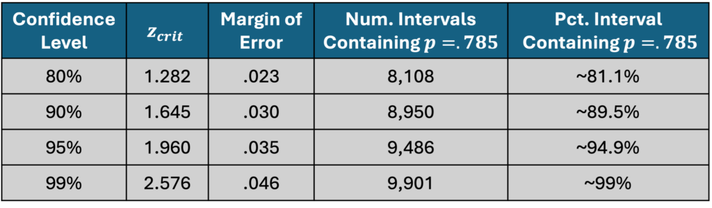
Evidently, there is pretty good agreement between the theoretical confidence on the left and the empirical confidence on the right. As you take more and more samples, the numbers on the right will get even closer to their counterparts on the left.
There you have it. The next time you make a confidence interval, you’ll understand what it means: if you take millions of samples and construct X% confidence intervals for each sample, then approximately X% of those confidence intervals will contain the true population parameter. I hope that this was helpful. R code for the simulation is available on request. Please comment with any questions or suggestions for future posts.
The post What is a confidence interval? appeared first on Paul Cornwell.