


Introduction to Simulation

I know that lots of my future posts are going to be about simulation. To introduce the topic gently, I’d like to start with a simple simulation that can be done in Excel. In short, a simulation is a model of a system that involves randomness. Most simulations use a computer, although the simulation I’ll talk about today was originally done by dropping a needle on the floor.1 Simulations are handy because they can give you a good idea of what might happen in situations that are hard to analyze. As they say, “‘Tis easier to verify than to figure out.” (They might not say that.) In this simulation, we’re going to approximate the mathematical constant π. Why π, you ask? Because the simulation is easy to set up, and we already know what the answer should be. Also, today is π-day, and what better way to celebrate?
But first, a quick aside on π. In college, I had a professor who, one day, quietly started writing out all the digits of π on the blackboard. Over the course of 3-4 minutes, he must’ve written out hundreds of numbers. Every so often, he would pause and scratch his chin, trying to recall the next part of the sequence. The whole class was amazed when he finally stopped writing. He then walked over to the left side of the board, drew a line after 3.1415 and said, “I know π up to here.”
Back to the simulation…Let’s start with a picture. Start by drawing a circle of radius 1. Put it in the middle of a 2D coordinate plane, so that its center is (0, 0). Next, circumscribe a square about the circle. Since the circle has radius 1, the square has side length 2, with corners at (+/-1, +/-1). Suppose you picked a random point within the square. Based on the picture below, it seems likely that it would also lie in the circle. However, it’s possible that the point could be near one of the corners of the square, in which case it would lie outside the circle. The exact probability of a random point lying in the circle is given by the ratio of the areas. Using high school geometry, we get:
^2}{2^2} = \frac{\pi}{4}.")
Since π is a little bigger than 3, there’s a little better than a 3 in 4 chance that a randomly selected point in the square will also lie in the circle. However, for this exercise, we’ll pretend that we don’t know the value of π. Instead, we will randomly generate a bunch of points in the square, verify whether each point lies in the circle, and then calculate the proportion of points which lie in the circle. Based on the equation above, should be equal to 4 times the proportion of points that lie within the circle. Notice that everything about this is simple: as long as you have the ability to generate random numbers, you don’t need any special math weapons. The rest is purely computational.

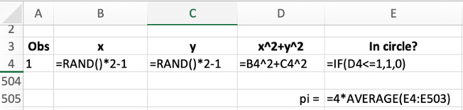
While you’ll want to use other coding languages or software for most simulations, Excel is perfectly fine for this one. The first step is to generate the random numbers. The Excel function RAND() generates a random number between and 0 and 1. If we multiply the output by 2 and subtract 1, we’ll get a random number between -1 and 1, as desired. Since we have x- and y–components, we must do this twice for each point. The next step is to see if the point lies in the circle. The circle is defined by the equation x^2 + y^2 = 1, and the interior of the circle by the condition x^2 + y^2 < 1. In Excel, we can use an if statement to return a value of 1, if the latter expression holds, and 0, if it does not. You can see the formulas in the screenshot below. I repeated this process for 500 points, and then took the average of the “In circle?” column. Out of 500 points, 396 were contained in the circle, which gives a proportion of 0.792. Multiplying this number by 4, we get our estimate π = 3.168. Not too shabby! If you’re playing along at home, you might have a slightly different answer. As I mentioned, I generated points 500. By the Law of Large Numbers, your answer should get closer and closer to π = 3.1415… as you generate more and more points.
This concludes today’s post. Please comment with questions or suggestions for future topics.
The post Introduction to Simulation appeared first on Paul Cornwell.
This simulation is an adaption of what’s known as the Buffon needle experiment, described in the 18th century by Georges-Louis Leclerc, Comte de Buffon. Make no mistake—the Comte was no buffoon. He was something of a polymath, whose work anticipated the theory of evolution.