


What does it mean to "train" a model?
A quick look at the algorithm used to tune parameters in linear regression.

Unless you’ve been living under a rock, you’ve probably noticed that AI mania has taken over the business world. As a result, the jargon of AI (and its cousins, machine learning, deep learning, etc.) has seeped into the mainstream. In this post, I want to talk about one buzzword in particular: what it means to train a model.
I’ll be working with a fake dataset that relates sales (in hundreds of thousands of dollars) to advertising spend (in thousands of dollars).

As a data analyst, the second thing you want to do is explore the data. (The first thing is to make sure that you understand what all the fields—i.e., variables—represent.)
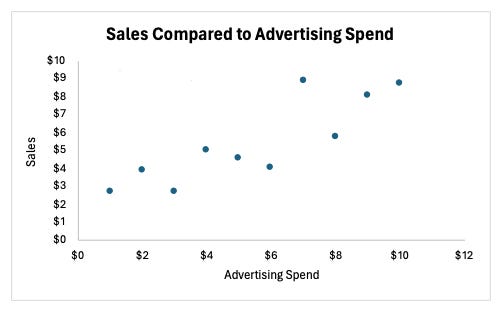
In this case, we see that sales increase as ad spending increases, and that the impact is fairly consistent across spending levels. We therefore might start by trying to fit a linear model to our data. This step of the modeling process is called model selection—deciding which type of model to use and which features to include. In real life, this decision would be a lot more complicated because there would be other variables, and the relationships would be less clear. You would also iterate on the model selection process by seeing how well different types of models perform on the dataset (or better yet, on a separate testing dataset).
Linear regression is an example of a parametric model. This means that it is entirely determined by one or more parameters. For simple linear regression, there are two parameters: slope m and intercept b of the line. Other machine learning models may have billions of parameters (e.g., the large neural networks you find in deep learning). Fundamentally, the training process for linear regression and deep learning is the same.
How to train your model
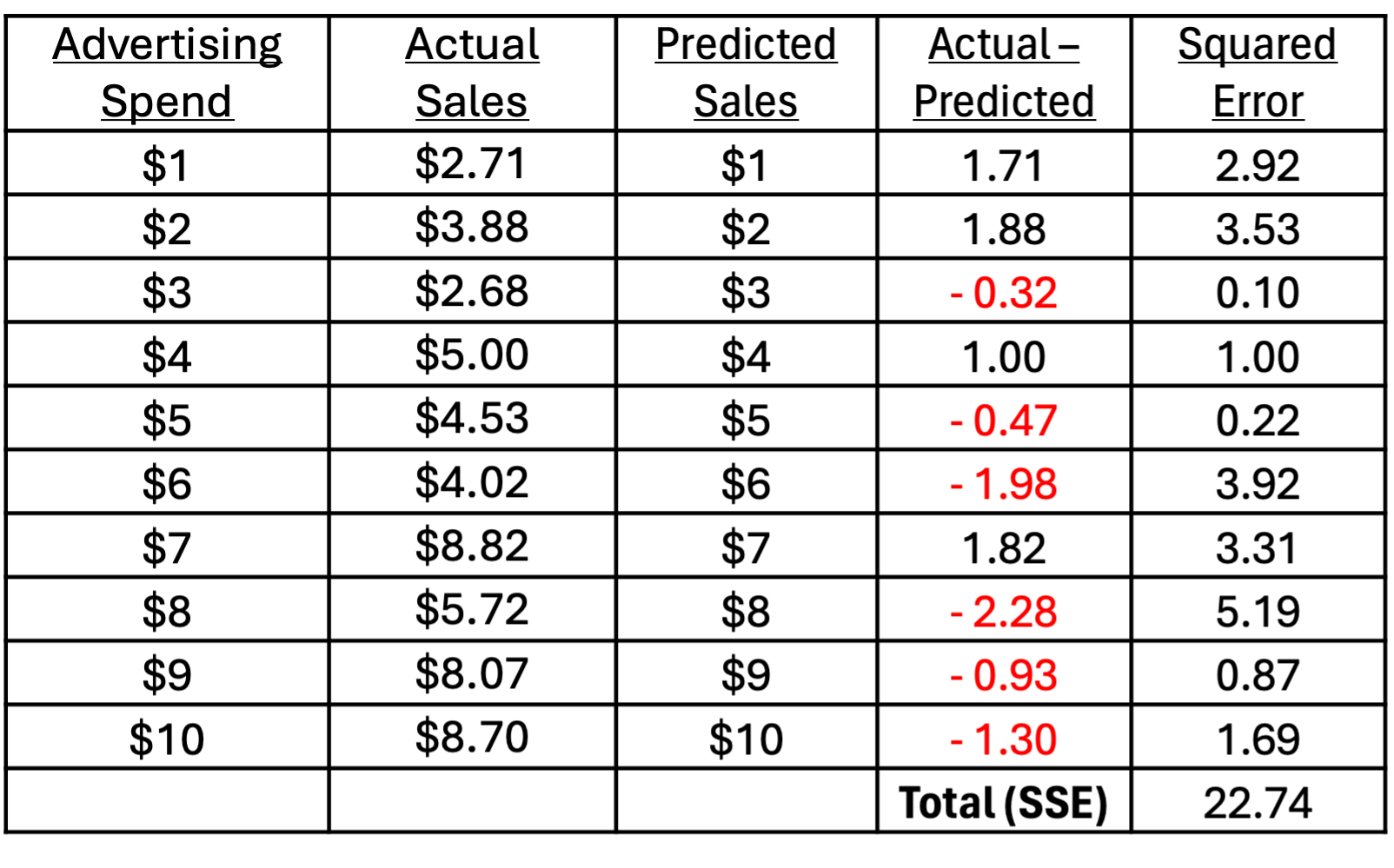
You might recall from statistics class that there is a formula for the slope and intercept of a linear regression model. (See the attached Excel.) Suppose you didn’t know that formula. How would you go about picking the slope and intercept? One thing you could do is just guess: say, m = 1 and b = 0. If you did that, you would end up with the following predictions for sales at each level of ad spend:

The next question is how do we go about assessing the quality of our predictions? The natural answer is to take the difference between the predicted and actual sales. That’s the right idea, although there is one problem: some of those deltas will be positive, and others negative. If you want to aggregate across ad spend levels, the positive and negative errors will offset. To fix that, we simply square the difference between predicted and actual sales before adding them up. The result is called the sum of squared errors (SSE). (You might wonder why we don’t take the absolute value instead. Let’s put a pin in that for now.)
The SSE gives us a metric—a number that allows us to evaluate the quality of our predictions. Larger errors mean a larger SSE, so our task is to find the values of m and b that minimize SSE. In math, this is called optimization. Although I’m focusing on simple linear regression, training any model amounts to an optimization problem.
We still haven’t addressed the elephant in the room: how do you find the values of the the parameters that minimize SSE? Since b and m could be anything, guessing randomly seems like a bad idea. Instead, let’s see if we can find a formula for SSE that works for any b and m:
To be fair, this isn’t pretty, but it does depend only on b and m. (The x’s and y’s are fixed.) In fact, if you group the terms together, you’ll see that SSE is a 2nd-order polynomial in m and b. The graph of SSE is a paraboloid—think of a satellite dish—which opens upward. Here’s a picture.
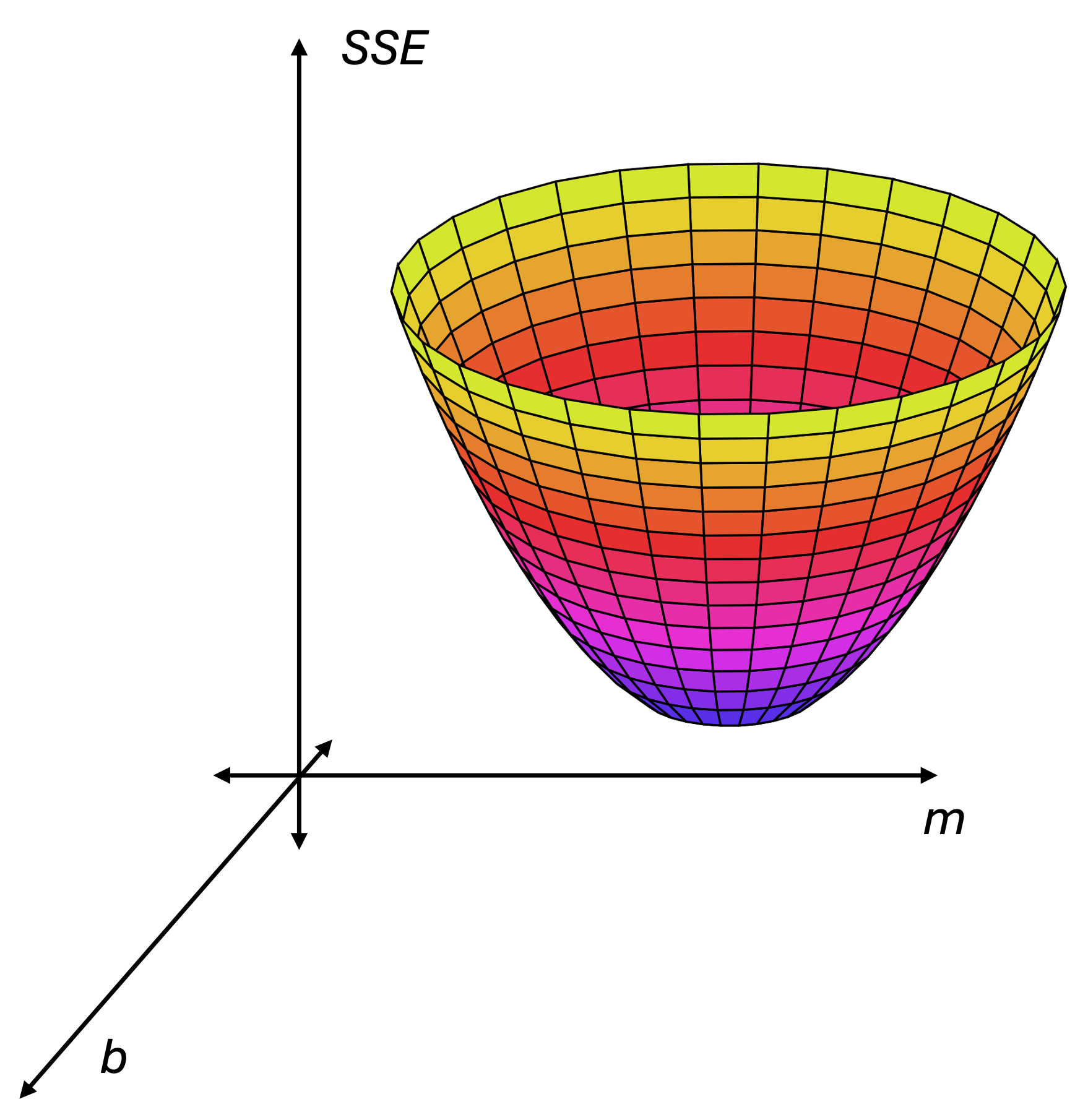
Minimizing SSE is all about getting to the bottom of that bowl. To explain how to do that, I’m going to simplify things a little bit. Let's pretend that we only have one parameter, b. Now, the graph of SSE looks like a parabola in the plane. Pick any point on the parabola and draw a tangent line—the straight line that just touches the curve at that point. The slope of the tangent line is found by taking the derivative of SSE with respect to b.1 Unless you're at the lowest point of the parabola, called the vertex, the tangent will have some slope. If you're far from the vertex, this slope will be steep.
To find the optimal value for b, begin by moving down that line a little bit towards the vertex. If you walk a short enough distance, you will still be very close to the parabola. Next, jump back up to the SSE curve at the same value of b and draw the new tangent line. You’ll notice that this line is less steep than the previous one. Once again, move a short distance towards the vertex and correct back to the parabola. If you repeat this process over and over again, then eventually, the tangent becomes almost flat. This indicates that you're nearing the vertex—the point where SSE is minimized. (If you accidentally overshoot the vertex, then on the next iteration, you’ll move in the opposite direction.) On a computer, you would stop this process once the slope of the tangent line got below some threshold, which would be a very tiny number.

Now, what if you go back to the case with two parameters (i.e., the satellite dish)? The same method works. The analog of the tangent line is the gradient, which is a vector that points in the direction in which SSE increases the fastest. (Walk in the opposite direction to get SSE to decrease as fast as possible.) Just like the slope of the tangent line is given by the derivative of SSE, the direction of the gradient is given by the partial derivatives of SSE (with respect to m and b separately). This method of following the tangent line/gradient to reach the minimum SSE is called gradient descent. The iterative nature of this method is why people use the word “training” for tuning parameters in models. The idea is that your model gets a little better each time you adjust b.
What about deep learning?
I mentioned earlier that the fundamental idea of model training is the same for regression and much larger (in terms of number of parameters) models such as you find in deep learning. Although I stand by that statement, the devil is in the details. First of all, computing the gradient means taking one derivative for each of the parameters that you have. As the number of parameters gets large, this becomes very taxing on the computer. The bigger issue, however, is what the loss function looks like for neural nets. In linear regression, the SSE graph—also called the “response surface”—always has that bowl shape, so there is a unique parameter value that minimizes SSE. If you implement gradient descent, it will get you to the bottom of the bowl (albeit slowly, in some cases).2 In contrast, neural nets have “lumpier” response surfaces due to the parameters being arranged in layers and some nonlinearities, which create complex interactions. In brief, gradient descent will get you to the bottom of whatever bowl you start in, but there will be other bowls that have deeper bottoms.

To address the above issues, researchers have developed (or repurposed) several numerical optimization concepts: stochastic gradient descent, batch processing, momentum, and more. In my opinion, the explosion of deep learning since the early 2010s is more of a hardware story than an algorithm one. No matter how you slice it, training a model that has billions of parameters is a monumental task. The broad applicability of machine learning and AI today is really enabled by recent hardware advances, such as GPUs. (If you don’t believe me, check out NVIDIA’s stock price.)
Back to our simple linear regression
We now know what it means to train a model: once you have a model paradigm (e.g., linear regression with one predictor, ad spend), you continually improve your model by adjusting the parameters in a way that minimizes your prediction errors. Here is a schematic of the training process.

The main thing I want you take away from this post is that model training is an optimization problem. In fact, I think optimization is the math problem of the 21st century for exactly this application. If you don’t have any weekend plans, you can try to set up and solve this optimization problem yourself. For example, you may be familiar with Solver in Excel. In the attached workbook, I solve the problem of minimizing SSE with Solver and compare it to Excel’s regression output and the regression formula. Thank you for reading. Please post any comments or questions and share with people who may enjoy the article.
This is why we use squared errors instead of absolute value. The derivative of the absolute value function is not defined at the minimum error (shaped like a “V”), so a calculus-based approach wouldn’t work well.
There’s one gotcha here: you have to choose the learning rate appropriately, which can be tricky. The learning rate is the size of the step that you take along the tangent line. There are a ton of papers written about this topic alone, especially adaptive learning rates (i.e., those that change over time).