DIY Mortgage Table
If you haven’t gone through it yet, one of the most exhilarating steps of the home-buying experience is shopping for mortgages. In this post, I’m going to show you how you can build your own mortgage table. (For the lazy among you, feel free to skip to the bottom for the completed version.) A mortgage table tells you what your monthly mortgage payment would be for different home prices, down payments, and interest rates. It also tells you how much of your loan you’ve paid off at a given point in time. That information is important if you want to refinance your mortgage or pay it off early. Use this tool to get a better handle on how much house you can afford. In no time at all, you’ll be longing for your renter days, as you shell out two grand to replace your water heater.
Disclaimer: This table does not include your monthly escrow payments (homeowners insurance, property taxes, mortgage insurance, etc.). Your actual payment could be 10-40% higher to account for escrow payments.
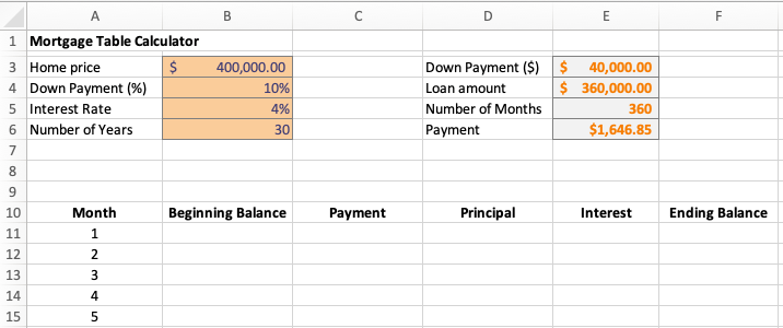
Step 1: Open a new Excel workbook. At the top, make 4 input cells (home price, down payment %, interest rate, number of years) and 4 calculated cells (down payment $, loan amount, number of months, payment).
Google “current mortgage rates” to find the prevailing interest rates from a number of sources. (Spoiler alert: they’re much higher than 4%.) Here are the formulae you need:
Down payment ($) = (Home price)*(Down Payment %). Alternatively, you can type a dollar amount directly into this cell (e.g., if you saved a certain amount for the down payment).
Loan Amount = (Home price) – (Down payment $)
Number of Months = 12 * (Number of Years)
Payment = PMT( (Interest Rate)/12, (number of months), -(Loan amount)). With the setup shown above, the exact formula would be =PMT(B5/12, E5, -E4). How this formula works is the subject of a future post.
Step 2: A few rows below your inputs, create 6 column headers: Month, Beginning Balance, Payment, Principal, Interest, Ending Balance.
In the Month column, start typing the integers from 1 up to the number of months.1 Typically, this will be 360, unless you’re a Dave Ramsey person, in which case it might be 180 (15 years). Excel pro tip: start with 1, 2, and 3, and then highlight those 3 cells. If you hover over the bottom right corner of the cell with 3 in it, Excel will recognize the pattern, and you can drag down the list until the end of the loan.
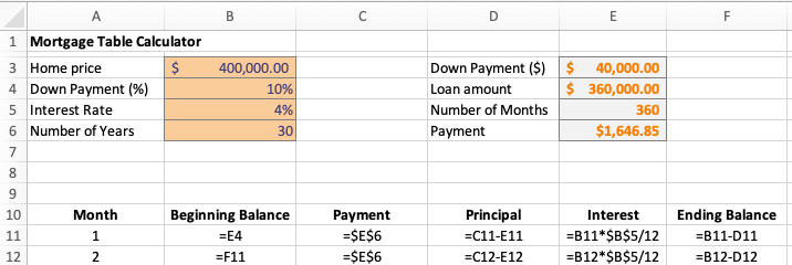
Step 3: Fill out the first month. This is where we’ll begin to see how everything works. “Beginning Balance” refers to the outstanding loan balance at the beginning of the month. You haven’t made any payments yet, so this is just equal to the loan amount (cell E4). The payment is exactly the payment you calculated earlier (cell E6). This will be the same every month.
Every mortgage payment you make has two components: principal and interest. Interest is interest, and principal is the portion of the loan that you are repaying. Skip Principal for a second. How much interest do you owe? The interest rate that you’re quoted is a nominal (finance speak for “fake”) rate that approximates your yearly interest. The actual monthly interest is one twelfth of this, so the interest you pay is (beginning balance)*(interest rate/12) (=B11*(B5/12)). Notice that we also divided by 12 in the PMT formula earlier.
Now back to principal. This is the component of the loan that you’re actually repaying with your monthly payment. It is calculated as a residual: Principal = (Payment) – (Interest) (cell C11 – E11). If you really want to feel sad, look at how big the interest payment is compared to the principal payment in the first month. Over time, the proportion of your payment that goes towards principal will increase. Finally, the ending balance is how much remains on the loan after you’ve made your payment. It is given by: Ending Balance = (Beginning Balance) – (Principal) (cell B11 – D11).
Step 4: Fill out the rest of the table. In month 2 (row 12), the Beginning Balance is just the Ending Balance from the previous month (cell F11). You might have to adjust the formula if the bank gives you a valued customer rebate, but that’s rare. The payment in month 2 is exactly the same as before (cell E6). Since it won’t change moving forward, you may as well write $E$6 to fix the cell reference. The same goes for the interest rate, so set Interest = ($B$5/12)*(B12). (Remember, interest is calculated based on the beginning balance for each month.) The Principal and Ending Balance formulae can just be copied from the previous row (no $ here). They should be (C12 – E12) and (B12 – D12), respectively.
The two pictures below show the formulae and outputs for the first two months. To fill out the rest of the table, highlight cells B12:F12 (the second month) and drag the formulas down until the last month. If you did everything correctly, the ending balance for the very last month should be exactly $0. Isn’t it nice when the answer key is built into the test? In contrast to first few months, you’ll see that almost your entire payment goes to paying off principal towards the end of the loan.
Now you have your very own mortgage table. As promised, there is a completed table below if you want to skip doing the work. In the completed version, I named some of the input cells to make the formulae more intelligible. I also added the sum of the payment, principal, and interest columns. You should see that the total principal paid is equal to the loan amount, and that that the sum of the payments is equal to the sum of the interest and principal columns. I recommend sitting down before you look at the sum of the interest column.
I hope that this post was enjoyable and helpful. Please comment with questions or requests for future posts.
The post DIY Mortgage Table appeared first on Paul Cornwell.
The only downside of doing this in Excel is that the list of months isn’t dynamic. That is, if you switch the length of the mortgage, you’d have to add or delete rows manually. If you pick a loan length that is less than 30 years, you can also just ignore the rows after the loan is repaid.


